ARIMA Explained: How the Autoregressive Integrated Moving Average Model Predicts Market Trends

In the ever-evolving realm of time series forecasting, the Autoregressive Integrated Moving Average (ARIMA) model stands out as a fundamental yet powerful tool. In this article, I will delve into the intricacies of ARIMA models, illuminating their components, mathematics, and practical application. As someone who has spent years analyzing time series data, I understand both the theory and its application in real-world scenarios. It’s this synthesis of experience and knowledge that I bring to the table in this exploration of ARIMA.

Introduction to ARIMA Models

What is an ARIMA Model?

An ARIMA model is a statistical analysis model that leverages time series data to predict future points in the series. The acronym ARIMA stands for Autoregressive Integrated Moving Average. Each component plays a unique role: ‘Autoregressive’ indicates that the model uses the dependent relationship between an observation and several lagged observations; ‘Integrated’ means that the model accounts for the non-stationarity in the time series data by differencing; and ‘Moving Average’ involves the model using a relationship between an observation and a residual error from a moving average model applied to lagged observations.

As a practitioner, it’s essential to appreciate not just the mechanics behind ARIMA but also its versatility. I recall my initial encounter with ARIMA while working on forecasting sales for a retail company. The data appeared chaotic, but ARIMA revealed underlying patterns that were invaluable in our strategic planning.

The Importance of ARIMA Models in Time Series Analysis

The importance of ARIMA models in time series analysis cannot be overstated. With their ability to model complex data patterns, ARIMA serves as a staple in fields ranging from economics to meteorology. They allow analysts to make short-term forecasts confidently, enabling businesses to better manage inventory, staffing, and other critical operational elements.

Moreover, ARIMA’s flexibility in addressing both seasonality and trends makes it essential in the toolbox of any data analyst. Over the years, I’ve leveraged ARIMA models to guide decision-making processes in various industries, showing just how potent they can be when applied thoughtfully.

The Components of ARIMA Models

Understanding Autoregression (AR)

Autoregression is the first building block of ARIMA. Essentially, it specifies that the current value of the series is based on its own past values. This relationship is captured through the use of lagged values of the dependent variable. An autoregressive model of order p (denoted as AR(p)) uses the past p observations to predict future values.

In practice, I have often found that selecting the right lag order p is crucial. Too few lags can oversimplify the model, while too many can lead to overfitting. A well-balanced approach arises from analyzing the ACF and PACF plots to determine the appropriate number of lags to include.

Grasping the Concept of Integration (I)

Integration refers to the differencing of observations in the time series to ensure it becomes stationary. This is essential because most statistical modeling techniques assume that the underlying data is stationary – meaning its statistical properties do not change over time.

To achieve a stationary series, one might compute the difference between consecutive observations. This step not only stabilizes the mean of the time series but also helps in enhancing the predictive ability of the model. In my experience, I’ve seen datasets significantly improve in terms of predictability post-differencing.

Deciphering Moving Average (MA)

The Moving Average component allows for the incorporation of the dependency between an observation and a residual error from a moving average model. It essentially uses past forecast errors to influence future predictions, which helps in smoothing out the noise in the data.

Specifically, an MA model of the order q (MA(q)) involves the relationship of the current observation with q previous errors. Finding the right q value can make a substantial difference in the model’s performance. This nuance often requires patience and extensive validation through techniques like cross-validation.

The Mathematics Behind ARIMA Models

The Role of Differencing in ARIMA Models

Differencing is a critical mathematical operation within ARIMA that assists in rendering the time series stationary. By calculating the difference between consecutive observations, we can effectively remove trends or seasonality from the data.

For instance, given a series \( Y_t \), the first difference \( Y_t – Y_{t-1} \) helps identify how the values change over time. This transformation must be handled with care, as too much differencing can lead to the loss of important patterns. In my analytical journey, employing the right degree of differencing often marked a turning point in model performance.

The Significance of Autocorrelation and Partial Autocorrelation

Autocorrelation functions (ACF) and partial autocorrelation functions (PACF) are vital tools for determining the appropriate parameters of ARIMA models. The ACF helps in identifying the order of the MA component, while the PACF is utilized to identify the order of the AR component.

In practice, I’ve relied on these plots to inform critical decisions during model selection. Understanding the intricacies of autocorrelation can sometimes lead one to discover unexpected relationships within the data, further enhancing the model’s robustness.

Building an ARIMA Model

Identifying the Order of an ARIMA Model

Identifying the correct order of an ARIMA model (usually represented as ARIMA(p,d,q)) requires a blend of analytical skills and subject-specific knowledge. Analysts typically start by analyzing ACF and PACF plots, conducting tests like the Augmented Dickey-Fuller test for stationarity, and systematically employing differencing methods.

In my experience, a combination of domain knowledge and statistical tests provides the most accurate results. I have often found that understanding the subject matter enriches the interpretation of the analytical outputs, leading to better-informed modeling decisions.

Estimating and Fitting the Model

Once the order is identified, the next step is to estimate the parameters of the model. This is commonly achieved through Maximum Likelihood Estimation (MLE) or Bayesian methods. After fitting the model, it’s pivotal to evaluate its performance through residual analysis.

In my early days, I was cautious about blindly trusting the fitted model without assessing its residuals. It’s an essential step; a good model should have residuals that resemble white noise. Taking this step would save countless hours in future forecasting inaccuracies.

cEvaluating the Performance of ARIMA Models

Diagnostic Checks for ARIMA Models

Diagnostic checks involve verifying whether the assumptions of the ARIMA model hold true. This includes examining ACF and PACF of residuals to ensure they do not exhibit autocorrelation.

In my practice, conducting thorough diagnostic checks has often revealed underlying issues which required fine-tuning the model. It’s not uncommon for a model to seem like a perfect fit superficially, only to unveil significant residual autocorrelation upon closer inspection.

Forecasting with ARIMA Models

Finally, once the ARIMA model is deemed satisfactory, we can utilize it for forecasting future observations. It’s crucial to maintain an eye on model accuracy and periodically reassess the model with new data to ensure its effectiveness.

Throughout my journey, I’ve learned that continuous learning and adaptation are key components to mastering ARIMA forecasting. Each dataset provides an opportunity to enhance one’s skills and refine forecasting acumen.

Frequently Asked Questions (FAQ)

1. What is an ARIMA model used for?
   

   An ARIMA model is primarily used for forecasting time series data where past values are predictive of future values.

2. How do I determine the order of an ARIMA model?
   

   The order can be determined using statistical plots such as ACF and PACF, along with tests for stationarity.

3. What preprocessing steps are necessary before building an ARIMA model?
   

   Key preprocessing steps include ensuring the data is stationary, handling missing values, and possibly removing outliers.

4. How do I evaluate the performance of an ARIMA model?
   

   Performance evaluation can be achieved through residual analysis, ACF/PACF plots of residuals, and accuracy metrics like RMSE.

In closing, mastering ARIMA models is a journey that combines statistical rigor with practical application. With a profound understanding of its components and a structured approach to analysis, one can harness the power of ARIMA to unlock significant insights in time series data.

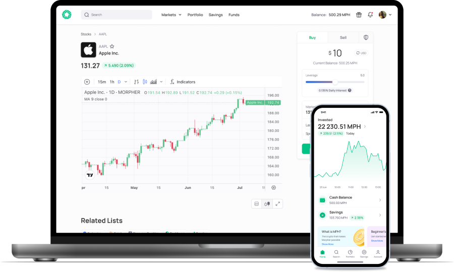
Now that you’ve gained insight into the power of ARIMA models for time series forecasting, imagine the possibilities when you apply such analytical prowess to the world of trading. Morpher is the perfect platform to take your trading strategy to the next level. With its zero-comissions structure, infinite liquidity, and the ability to trade across a multitude of asset classes, Morpher empowers you to trade smarter and more efficiently. Whether you’re looking to invest fractionally, short sell without interest fees, or leverage your trades up to 10x, Morpher offers a revolutionary trading experience on the Ethereum Blockchain. Embrace the future of investing with Morpher. Sign Up and Get Your Free Sign Up Bonus today and start transforming your trading journey.

Disclaimer: All investments involve risk, and the past performance of a security, industry, sector, market, financial product, trading strategy, or individual’s trading does not guarantee future results or returns. Investors are fully responsible for any investment decisions they make. Such decisions should be based solely on an evaluation of their financial circumstances, investment objectives, risk tolerance, and liquidity needs. This post does not constitute investment advice.